library(tidyverse)
library(broom.mixed)
library(brms)
library(knitr)
set.seed(55432)
# list of files
dir1 <- "https://raw.githubusercontent.com/avehtari/ROS-Examples/master/ElectionsEconomy/data/hibbs.dat"
# EXAMPLE 1: GDP GROWTH AND ELECTION VOTE SHARE
# quick simple example, using bayes for a linear regression
# what is the impact of economic growth on incumbent vote share?
election <- read_delim(dir1, delim = " ")
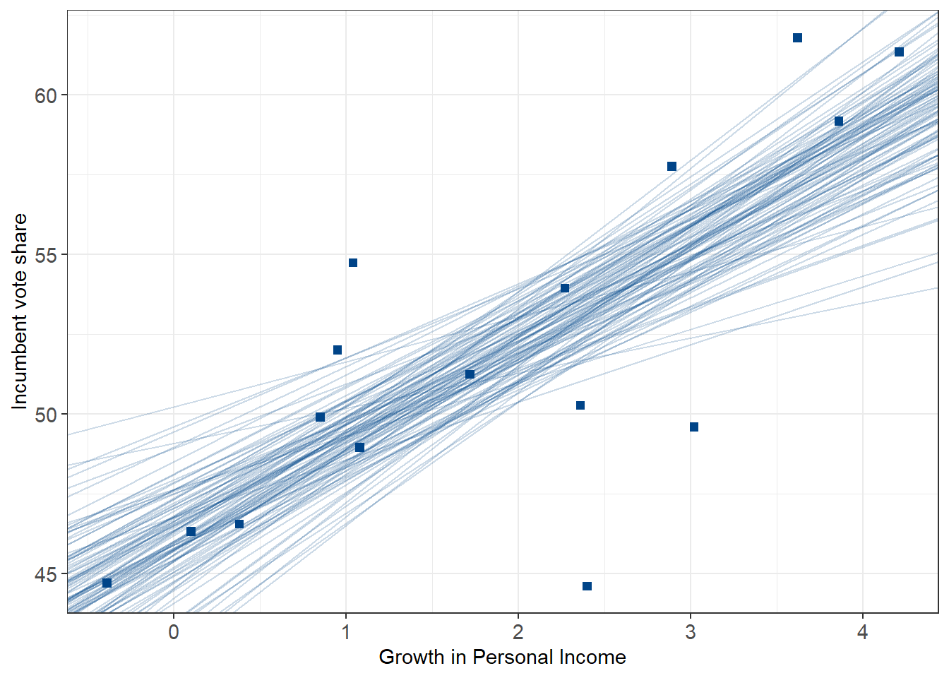
# plot 100 simulations from the posterior
plot_posterior <- function(fit){
M <- as.matrix(fit)
sims <- 100
sims_idx <- sample(1:nrow(M), size=sims)
model_sims <-
M[sims_idx, ][, c(1, 2)] %>% data.frame() %>% setNames(c("intercept", "slope"))
plot1.1 +
geom_abline(data=model_sims, aes(slope = slope, intercept = intercept), alpha = .2, color = '#004488')
}
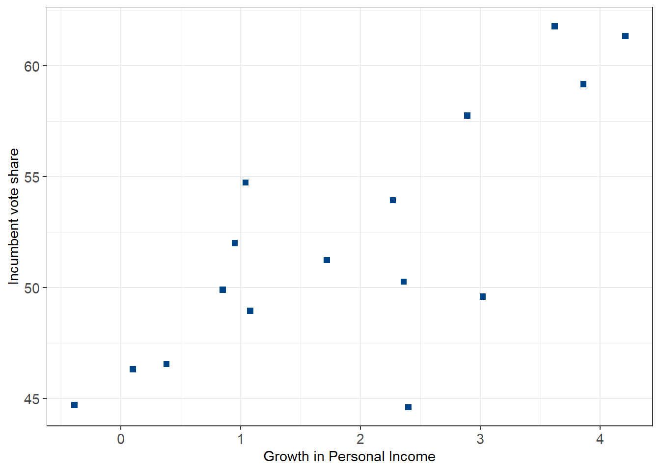
plot1.1 <-
  ggplot(election) +
  geom_point(aes(x = growth, y = vote), size = 2, shape = 22, fill = '#004488', color = '#004488') +
  labs(x = "Growth in Personal Income", y = "Incumbent vote share") +
  theme_bw() +
  theme(axis.text = element_text(size = 11))
plot1.1
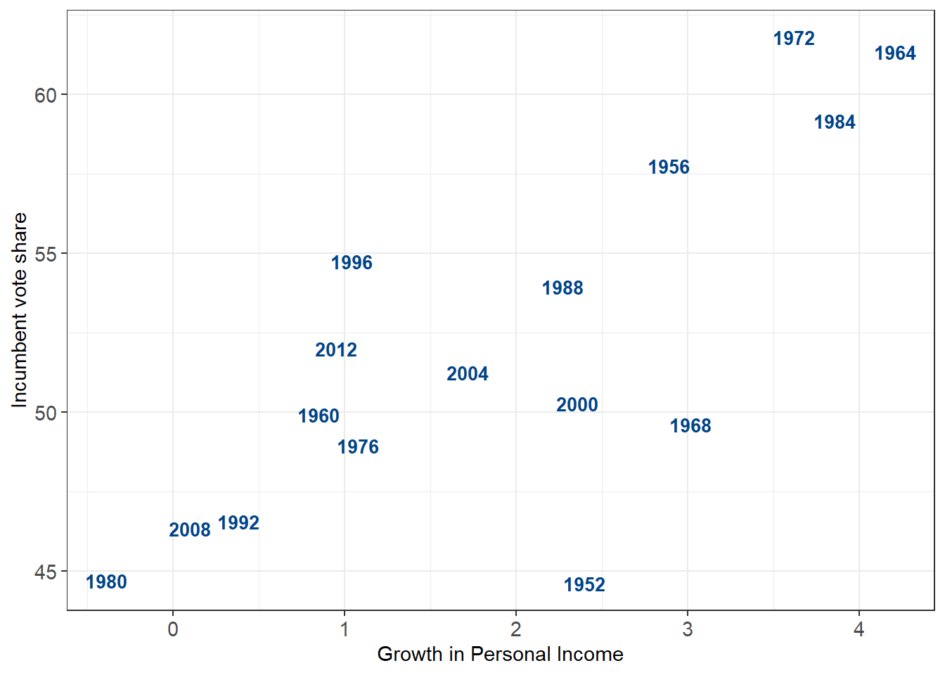
plot1.2 <-
  ggplot(election) +
  geom_text(aes(x = growth, y = vote, label = year), size = 3.5, fontface = 'bold', color = '#004488') +
  labs(x = "Growth in Personal Income", y = "Incumbent vote share") +
  theme_bw() +
  theme(axis.text = element_text(size = 11))
plot1.2
# let's regress!
fit2_prior <- c(prior(normal(3, 1), class = 'b'))

# model 1 has default (flat) priors on betas
# 1 percentage point in growth is associated with ~ 3% increase in vote share
fit1 <-
  brm(vote ~ growth,
      data = election,
      family = "gaussian",
      file = "hibbs_fit1.Rdata")
tidy(fit1) %>% kable(digits = 2, caption = "Flat prior")
# same model, with much tighter priors
# assuming a mean effect of about 2.5% +- 1.5%
fit2 <-
  brm(
    vote ~ growth,
    data = election,
    family = "gaussian",
    prior = fit2_prior,
    file = "hibbs_fit2.Rdata"
  )
tidy(fit2) %>% kable(digits = 2, caption = "Informative prior")
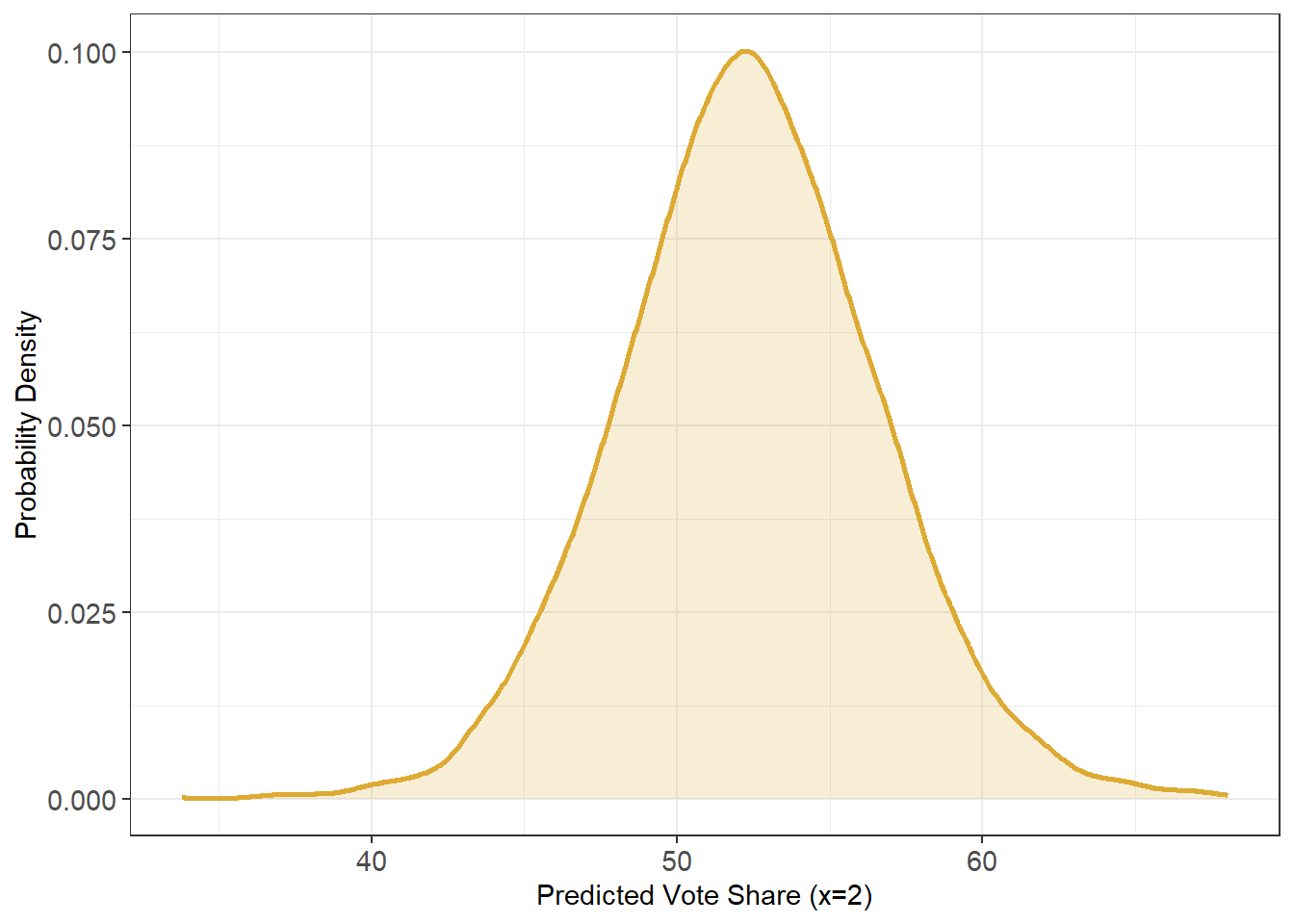
# what is the predicted vote share given a 2% growth rate?
# ~52%, but with a pretty big margin of error
newgrowth = 2.0
newprobs = c(.025, .25, .75, 0.975)

pred1 <- posterior_predict(fit1, newdata = data.frame(growth=newgrowth))

ypred = mean(pred1)
ypred_quantile = quantile(pred1, newprobs)


ggplot(data.frame(x = pred1)) + geom_density(aes(x = x), linewidth = 1, color = '#DDAA33', fill = '#DDAA33', alpha = .2) +
  labs(x = "Predicted Vote Share (x=2)", y = "Probability Density") +
  theme_bw() +
  theme(axis.text = element_text(size = 11))
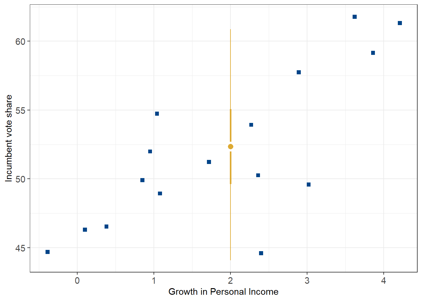
# plot the 50% and 95% credible intervals for the point estimate of 2% growth
plot1.1 +
  annotate(geom = "linerange", x = newgrowth, ymin = ypred_quantile[2], ymax = ypred_quantile[3], color = '#DDAA33',  linewidth = 1) +
  annotate(geom = "linerange", x = newgrowth, ymin = ypred_quantile[1], ymax = ypred_quantile[4], color = '#DDAA33') +
  annotate(geom = "point", x = newgrowth, y = ypred, fill = '#DDAA33', color = 'white', stroke = 2, size = 3, shape = 21)
plot_posterior(fit2)