outcome_table <- data.frame(
  id = c("control", "control", "treat", "treat"),
  time = c(0, 1, 0, 1),
  treat = c(0,0,1,1),
  count = c(447, 435, 729, 617)
)Crime Prevention and Difference-in-Differences
I was recently scanning through some posts on my linkedin page, and saw something interesting (or at least more noteworthy than the 1000 rage-bait or AI posts). This was a crime report from the city of Cape Town reporting on a new anti-crime initative. In my academic life I used to do similar work like this with the city of Detroit. My dissertation, in fact, focused on estimating the impact of CCTV cameras on crime at different types of businesses.
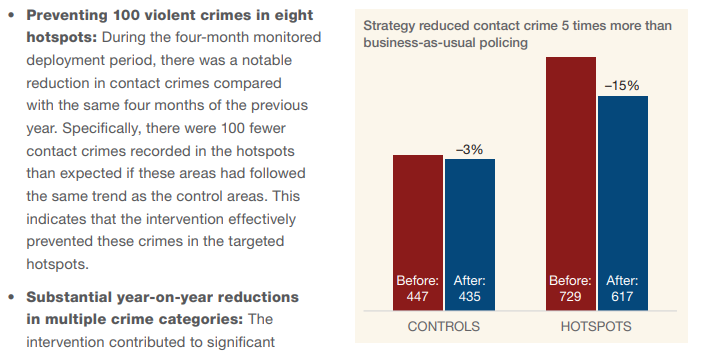
But I digress. I was just scanning the report and saw this at the top of the document:

This reminded me of the days when I used to teach graduate-level research methods courses about causal inference. This table is actually one of the most common types of estimations done. A “control” area (that gets no special attention by police), a “treatment” area (that gets some kind of new focused attention by police), and two time periods (pre-intervention and post-intervention). In the parlance of causal inference we can consider this the simplest kind of difference-in-differences problem.
Difference-in-Differences
What is difference-in-differences (DiD)? Well, to keep it brutally short, I’ll rely on the definition provided by some leading folks in DiD(Baker et al. 2025):
A basic DiD design requires two time periods, one before and one after some treatment begins, and two groups, one that receives a treatment and one that does not. The DiD estimate equals the change in outcomes for the treated group minus the change in outcomes for the untreated group: the difference of two differences.
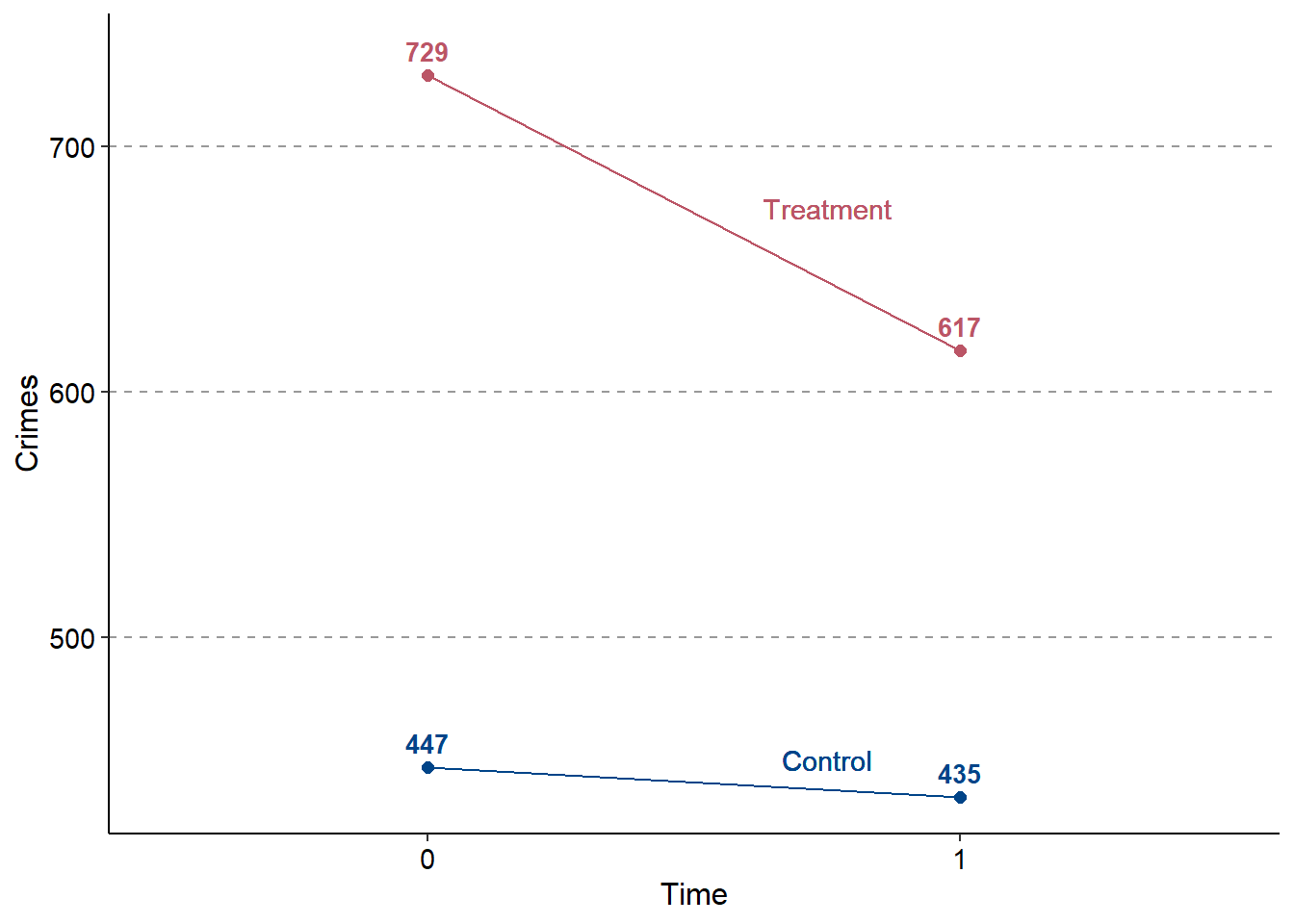
Emphasis mine. Let’s review the example from the Cape Town report briefly. There are two period, two groups, and 4 values for number of crimes. We can construct this in R quite easily. First, I’ll create a dataframe to hold the necessary information. You’ll note that I add variables for time period (where 0 is pre-treatment and 1 is post-treatment), and a variable for treatment group (either 0 for control and 1 for treatment).
And now using these data we can plot the slopes of the two periods for the two groups:

Computing the setup for this type of DiD model is actually very simple. A two-group, two-period model is often canonically known as a 2x2 DiD model. When I used to teach, I would often explain that most DiD models (and, by extension, most of statistics) is essentially fancy averaging. Therefore, computing the DiD estimand from a 2x2 model requires only a little simple math, which we can supplement with some functionality in R.
If we want to directly compute this in R, we can just use the lm function to do it all for us. lm in R sets up a linear regression model, where we provide an indicator for time (pre, post), and an indicator for treatment group (control, treat). The value that we are interested in is the number of crimes in the treatment group, in the post-treatment period, after subtracting out the prior differences in groups. The DiD estimand is simply the interaction between the treatment indicator and the time period:
Code
lm(count ~ time * treat, data = outcome_table)
Call:
lm(formula = count ~ time * treat, data = outcome_table)

Coefficients:
(Intercept)         time        treat   time:treat
        447          -12          282         -100
We see a few things here:
- The
(Intercept)which is the number of crimes whentime=0,treat=0andtime:treat=0. So this is the number of reported crimes in the control group in the pre-treatment period, which is \(447\). timewhich is the change in crime for the control group fromtime=0totime=1. Here this is \(-12 = 435-447\)).treatis the difference in crimes between the treated and control group whentime=0. Here we see this is simply \(282 = 729-447\)- And finally the DiD estimand, which is the number of crimes in the treatment group in the post-treatment period, subtracting out the prior differences in the pre-treatment period. Here we see it is \(-100\) which means we estimate that there were 100 fewer crimes in the treatment area relative to the control area.
A caveat here: typically we the treatment and control groups are averages of multiple units (e.g. neighborhoods or police beats). Since we only have access to the aggregated table we can’t compute variances or test-statistics because the model is fully saturated (4 parameters for 4 data points).
Summary
So I’m not introducing anything really new here - but just posting something that piqued my interest. I still see a ton of work using DiD designs (whether the authors are aware of it or not). Sometimes I find looking at the most basic version of a model design is often helpful before working on increasingly more complex ones. For example, models that account for staggered treatment implementation and treatment variation.
This barely scratches the surface, so if you are actually interested in this, I’d suggest a few difference resources: