# scale input attributes
X <- df[, 2:7]
X <- scale(X)

# compute NN distance between all points
# set n neighbors
k = 5

# compute k nearest neighbor distances
# using kd-trees
d <- RANN::nn2(X, k = k+1)
d <- d[[2]][,1:k+1]Part 2: The K-nearest neighbor anomaly detector
This is the second part of a 3-part series. In the previous post I talked a bit about my desire to work on building the pieces of an outlier ensemble from “scratch” (e.g. mostly base R code with some helpers).
In the first post I talked about my approach building a principal components analysis anomaly detector. In this post I’ll work on the K-nearest neighbors anomaly detector using the same base data.
To date, the three parts of the ensemble contain:
- “Soft” principal components anomaly detector
- K-nearest neighbors anomaly detector
- Isolation forest or histogram-based anomaly detector
Creating the KNN anomaly detector
Defining distance
In a way, the K-nearest neighbors anomaly detector is incredibly simple. To compute the anomalousness of a single point we measure its distance to its \(k\) nearest neighbors. We then use either the maximum or average distance among those \(k\) points as its anomaly score. However, there is some additional complexity here regarding the choice of \(k\) in an unsupervised setting - but we’ll get to that in a moment.
One issue is that computing all pairs of nearest neighbors has \(O(N^2)\) time complexity. However, we only need to know the number of nearest neighbors up to our value of \(k\). Therefore, we can avoid computing nearest unnecessary distances by applying more efficient algorithms - like k-d trees. In the case for \(k\) nearest neighbors the time complexity is \(O(N * log(N)\). The RANN package in R does this fairly efficiently. We’ll use the same data as in the previous post for this example.
You will notice that we set \(k\) to \(k+1\) to avoid calculating the nearest-neighbor distance to the each point itself (which is always zero). The nn2 package gives us the Euclidean nearest-neighbor distances for each point arranged from nearest to farthest. For example if we look at the top 3 rows of the distance matrix we see:
Code
d[1:3,] [,1] [,2] [,3] [,4] [,5]
[1,] 0.1457822 0.3123632 0.3311984 0.3641609 0.3726815
[2,] 0.5261689 0.6887312 0.9636189 1.0087124 1.0097114
[3,] 0.2874466 0.3044159 0.3723676 0.4139428 0.4251863Which gives us the standardized (Z-score) distance to the \(k\) nearest neighbor of point \(i\). Now all we need to do is decide on how we will summarize this distance.
Distance Measures
We have a few options for distance measures. The most common, and simplest to understand arguably, is to compute a score based on the distance to each observations farthest \(k\) neighbor (so if \(k=5\) the score is the largest distance among those 5 neighbors). We can accomplish this by just getting the max value from each row.
anom_max <- apply(d, 1, max)We also have another option. Rather than choosing the maximum of the 5 nearest neighbors, we can average over a larger number of neighbors. This has the advantage of removing some of the variance implicit in the choice of \(k\). For example, imagine the distance to the 6 nearest neighbors of one point are \([1, 2, 5, 7, 8, 100]\). If we chose \(k=5\) we would miss the obvious outlier that would have been found had we instead chosen \(k=6\). A good alternative to is set \(k\) much higher and get the average of all neighbors within that range. Here, we might set \(k\) to 20 and average over the distances.
anom_mean <- adKNN(d, k = 20, method = "mean")In many cases there will be very strong overlap between the two metrics, but in my personal experience I find that in unsupervised cases it is usually better to err on the safe side and go with metrics that do not depend on a single decision (hence, the entire purpose of outlier ensembling!)
Like before we can specify a cut-point to flag outliers. Here, it might be reasonable to set it to the highest 5% of anomaly scores. Unfortunately, there’s not necessarily a clear p-value available here like there was with the PCA anomaly detector. Ideally, if we have some prior information about the expected amount of contamination we could use that as our threshold instead. The plot below displays the 10 observations with the highest anomaly scores. The values flagged here look very similar to the ones that were identified by the PCA anomaly detector as well, which should give us some confidence.
Code
scored_data <- data.frame(df,anom_mean)

flag <- scored_data$anom_mean >= quantile(scored_data$anom_mean, .95)

ggplot() +
  geom_point(data = scored_data, aes(x = stay_len, y = diff), color = '#004488', size = 2, alpha = .25) +
  geom_point(data = scored_data[flag,], aes(x = stay_len, y = diff), color = '#BB5566', size = 2.5) +
  labs(x = "Stay Length", y = "Avg. Payment Difference") +
  theme_minimal() +
  theme(axis.text = element_text(size = 12),
        axis.title = element_text(face = "bold"))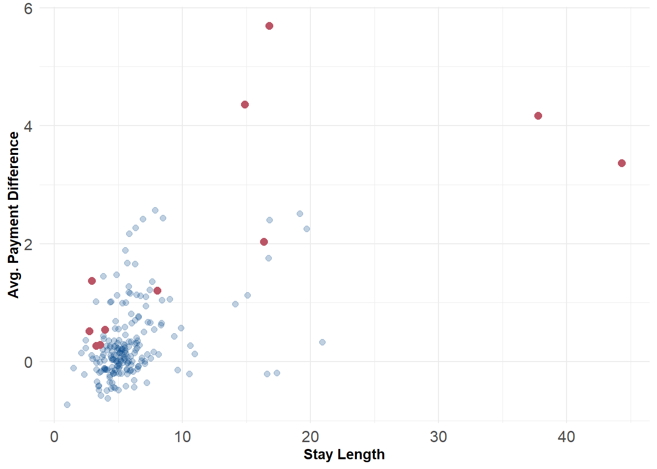
KNN Anaomaly Detector: Example Function
Here’s a minimal working example of the procedure above. As we build our ensemble, we’ll come back to this function later.
Code
# Run a principal components anomaly detector
adKNN <- function(X, k = 5, method = 'max'){

  # compute k nearest neighbor distances
  # using kd-trees
  d <- RANN::nn2(X, k = k+1)
  d <- d[[2]][,1:k+1]

  # aggregate scores
  if(method == 'max')
    anom <- apply(d, 1, max)
  else if(method == 'mean')
    anom <- apply(d, 1, mean)
  else
    print("Function not found")

  return(anom)

}