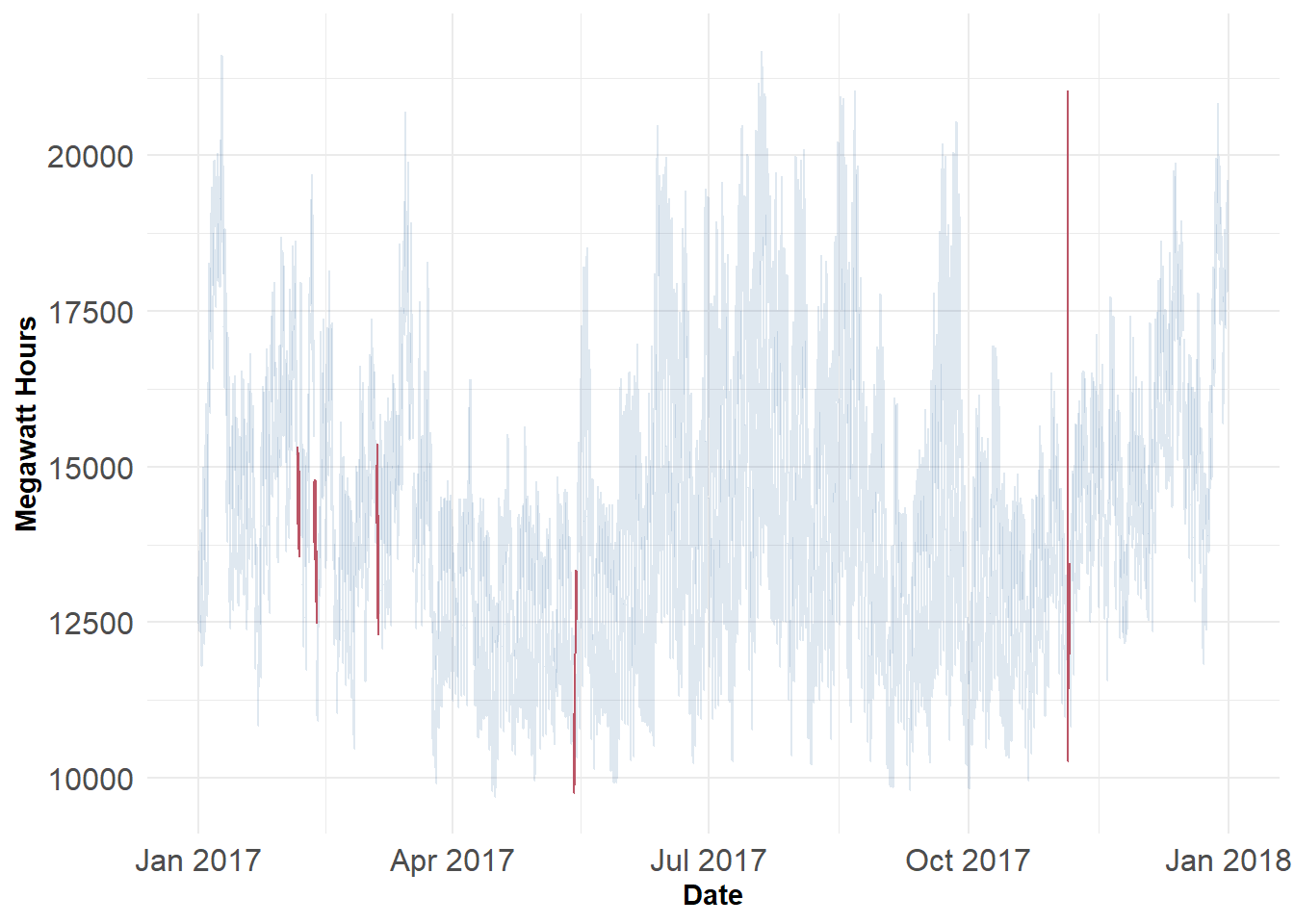
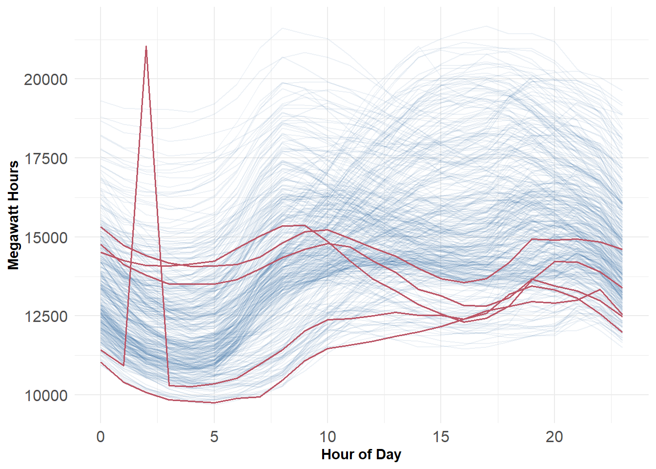
Anomaly Detection for Time Series

An Unsupervised Approach to Time Series Anomalies

Identifying outliers in time series is one of the more common applications for unsupervised anomaly detection. Some of the most common examples come from network intrusion detection, mechanical processes, and other types of high-volume streaming data.

Of course, there are just as many proposed ways of identifying outliers from the simple (basic Z-scores) to the complex (convolutional neural networks). There are also some approaches that rely on more conventional tabular approaches. Rob Hyndman proposed a few approaches here and here showing how many high-volume time series can be compressed into a tabular dataset. The general idea is that you can decompose many time series into tabular observations by creating a large variety of features describing each series.

Featurizing a time series dataset

The data we’ll use is on hourly power usage for a large power company (American Electric Power). From this dataset we can perform some basic aggregation (to ensure that all timestamped values are on the same day-hour), then separate each set of 24 hours into their individual days. The goal here is to make it easier to look at hours within each day. The code below does a bit of this processing. Of course, working with dates is still always a pain, despite the improvements in R libraries.

Code

# Read data, convert to zoo
elec <- read_csv("AEP_hourly.csv") %>%
  group_by(Datetime) %>%
  summarise(AEP_MW = sum(AEP_MW)) %>%
  filter(year(Datetime) %in% 2017)

elec_ts <- zoo(x = elec$AEP_MW, order.by = elec$Datetime, frequency = 24)

# Split the hourly time series into daily time series
daily_ts_list <- split(elec_ts, as.Date(index(elec_ts)))

# Extract the first 24 observations of each daily time series
# dropping days with missing values
daily_24_ts_list <- lapply(daily_ts_list, function(x) {
  if (length(x) >= 24) {
    return(x[1:24])
  } else {
    return(NA)
  }
})

# Convert from list to dataframe
daily_24_ts_list <- purrr::discard(daily_24_ts_list, ~any(is.na(.)))

After converting the list of values to a data frame, we can proceed with the featurization. As we said before, we can use the tsfeatures library to decompose each day’s hourly values into a single observation. We can see this creates a data frame with 17 features, which correspond to various measures, including: autocorrelation, seasonality, entropy and other ad-hoc measures of time series behavior.

# Convert from list to dataframe, extract TS features
daily_24_ts_list <- purrr::discard(daily_24_ts_list, ~ any(is.na(.)))

# create time series features using `tsfeatures`
df <- daily_24_ts_list %>%
  tsfeatures(
    features = c(
      "acf_features",
      "stl_features",
      "entropy",
      "lumpiness",
      "stability",
      "max_level_shift"
    )
  ) %>%
  select(-nperiods,-seasonal_period)

Code

glimpse(df, width = 65)

Rows: 364
Columns: 13
$ x_acf1      <dbl> 0.8139510, 0.9318718, 0.9123398, 0.9173901,…
$ x_acf10     <dbl> 1.771656, 2.081091, 1.868137, 1.889912, 1.7…
$ diff1_acf1  <dbl> 0.6284980, 0.6181949, 0.6534759, 0.6194560,…
$ diff1_acf10 <dbl> 1.4141518, 0.7771648, 0.6910469, 1.0491669,…
$ diff2_acf1  <dbl> 0.3426413, 0.2082615, 0.3164917, 0.2786098,…
$ diff2_acf10 <dbl> 0.5009215, 0.2550913, 0.4214296, 0.2577332,…
$ trend       <dbl> 0.7256036, 0.9374949, 0.9377550, 0.9478148,…
$ spike       <dbl> 1.946527e-04, 4.715699e-06, 6.706533e-06, 4…
$ linearity   <dbl> 1.8002798, 3.6310069, 3.3908752, 4.1128389,…
$ curvature   <dbl> 0.4988011, -1.2265007, -2.0788821, -0.66100…
$ e_acf1      <dbl> 0.6719203, 0.6507832, 0.6513875, 0.6636410,…
$ e_acf10     <dbl> 1.4588480, 1.0862781, 0.9523931, 1.1326925,…
$ entropy     <dbl> 0.3585884, 0.5225069, 0.4962494, 0.3090901,…

Principal components anomaly detector

After doing this, we can proceed as a normal tabular data problem. The PCA anomaly detector that was detailed in an earlier post is an easy plug in here and is a natural fit for the problem. We have a lot of highly correlated measures that likely share a large amount of variance across a few dimensions. We can then weight the lower-variance dimensions higher to identify anomalous series. We’ll use the \(\chi^2\) distribution to derive a p-value, which we can then threshold for flagging outliers.

# Perform anomaly detection
anom <- adPCA(df)
p = sapply(anom, pchisq, df=ncol(df), ncp = mean(anom), lower.tail=F)

Results

We can see which series were flagged by the model by highlighting the series which were flagged at the \(p < .01\)

Code

# flag observations at p < 0.01
elec_plot <- elec %>%
  mutate(date = as.Date(format(Datetime, "%Y-%m-%d")),
         hour = hour(Datetime)) %>%
  left_join(scored_data) %>%
  mutate(flag = ifelse(p < 0.01,1,0))

ggplot(data = elec_plot, aes(x = Datetime, y = AEP_MW, group = date)) +
  geom_line(color = '#004488', alpha = .125) +
  geom_line(data = elec_plot[elec_plot$flag == 1,], color = '#BB5566') +
  labs(x = "Date", y = "Megawatt Hours") +
  theme_minimal() +
  theme(axis.text = element_text(size = 12),
        axis.title = element_text(face = "bold"))

Anamolous days are highlighted in red. Note the unusually high spike in late 2017.

We can also see what these anomalous series look like compared to the other series on a hourly basis. This plot clearly shows one series with a unusual early-morning spike, and several series with flatter trajectories compared to more normally expected seasonality - in particular, they are days with low power consumption in the afternoon when consumption is usually at its highest.

Code

ggplot(data = elec_plot, aes(x = hour, y = AEP_MW, group = date)) +
  geom_line(color = '#004488', alpha = .075) +
  geom_line(data = elec_plot[elec_plot$flag == 1,], color = '#BB5566', size = .7) +
  labs(x = "Hour of Day", y = "Megawatt Hours") +
  theme_minimal() +
  theme(axis.text = element_text(size = 12),
        axis.title = element_text(face = "bold"))

Anomalous days often have flatter curves and dip during high-load hours of the day.

Arguably this isn’t an ideal approach because each sub-series is only comprised of 24 observations. That means reliably identifying seasonality via the stl_features is questionable. In addition, this approach loses some information that comes from day-to-day correlations. It would probably be worthwhile testing this approach against something like STL decomposition.