library(tidyverse)
library(brms)

polls <- read_csv("https://projects.fivethirtyeight.com/polls-page/data/president_polls_historical.csv")
set.seed(8372)

# set up data, consistent with some other data sources
# this is just national polls
max_size = 5000
matchup = c("Harris", "Trump")

# get just harris-trump matchups
harris_trump <-
polls %>%
  group_by(poll_id, question_id) %>%
  summarise(all_reps = paste0(answer, collapse = ",") ) %>%
  filter(all_reps %in% c("Harris,Trump","Trump,Harris")) %>%
  pull(question_id)


# select data
# only national polls where trump-harris are the options
# remove polls that are overlapping

all_polls_df <-
polls %>%
  rename(pop = sample_size,
         vtype = population) %>%
  mutate(begin = as.Date(start_date, "%m/%d/%y"),
         end = as.Date(end_date, "%m/%d/%y"),
         t = end - (1 + as.numeric(end-begin)) %/% 2,
         entry_date = as.Date(created_at, "%m/%d/%y")) %>%
  filter(question_id %in% harris_trump,
         is.na(state),
         !is.na(pollscore),
         !is.na(numeric_grade),
         answer %in% matchup,
         end > as.Date("2024-06-01"),
         t >= begin & !is.na(t) & (vtype %in% c("lv","rv","a")),
         pop > 1,
         pop <= max_size) %>%
  mutate(pollster = str_extract(pollster, pattern = "[A-z0-9 ]+") %>% sub("\\s+$", "", .),
         pollster = replace(pollster, pollster == "Fox News", "FOX"),
         pollster = replace(pollster, pollster == "WashPost", "Washington Post"),
         pollster = replace(pollster, pollster == "ABC News", "ABC"),
         partisan = ifelse(is.na(partisan), "NP", partisan),
         method = case_when(
           str_detect(tolower(methodology) ,"online") ~ "online",
           str_detect(tolower(methodology) ,"phone") ~ "phone",
           TRUE ~ "other"),
         week = floor_date(t - days(2), unit = "week") + days(2),
         day_of_week = as.integer(t - week),
         index_t = 1 + as.numeric(t) - min(as.numeric(t)),
         index_w = as.numeric(as.factor(week)),
         index_p = as.numeric(as.factor(as.character(pollster))),
         n_votes =  round(pop * (pct/100))) %>%
  distinct(t, pollster, pop, party, .keep_all = TRUE) %>%
  select(poll_id, t, begin, end, entry_date, pollster, partisan, numeric_grade, pollscore, vtype, method, pop, n_votes, pct,party,answer, week, day_of_week, starts_with("index_"))

# remove overlapping polls
all_polls_df <-
  all_polls_df %>%
  group_by(entry_date, pollster, pop, party) %>%
  arrange(desc(entry_date), desc(end)) %>%
  slice(1)

# drop polls with combined 2-party vote share < 85%
low_vote <-
  all_polls_df %>%
  group_by(poll_id, entry_date, pollster, pop) %>%
  summarise(total_votes = sum(n_votes), .groups = 'drop') %>%
  mutate(prop = total_votes / pop) %>%
  filter(prop < .85) %>%
  select(poll_id, entry_date, pollster, pop)

all_polls_df <- anti_join(all_polls_df, low_vote)

# plot the 2 party pct
all_polls_df %>%
  ggplot(aes(x = t, y = pct, color = party)) +
  geom_point(aes(size = pop, fill = party),shape = 21, alpha = .2) +
  geom_smooth(aes(color = party)) +
  scale_color_manual(values = c("#00AEF3","#E81B23")) +
  scale_fill_manual(values = c("#00AEF3","#E81B23")) +
  scale_y_continuous(limits = c(30, 60)) +
  theme_minimal() +
  theme(legend.position = 'none')


# RUN MODELS
# -------------------- #

extract_posterior_predictions <- function(x){
  # get the median and 95% credible interval
  ypred <- posterior_predict(x)
  ypred <- apply(ypred, 2, quantile, probs = c(.025, .5, .975)) %>% round()
  data.frame(t(ypred)) %>% set_names(c("ymin","median","ymax"))
}

stack_extract_posterior_predictions_naive <- function(x1, x2, weights = c(.5, .5), return = "agg"){
  # average weighted predictions from two models
  pred1 <- posterior_predict(x1)
  pred2 <- posterior_predict(x2)
  pred_avg <- (pred1 * weights[1]) + (pred2 * weights[2])

  if(return=="agg"){
    ypred <- apply(pred_avg, 2, quantile, probs = c(.025, .5, .975)) %>% round()
    out <- data.frame(t(ypred)) %>% set_names(c("ymin","median","ymax"))
  }
  else if(return=="raw"){
    out <- pred_avg
  }

  return(out)
}

stack_extract_posterior_predictions <- function(x1, x2){
  # get the median and 95% credible interval
  ypred <- pp_average(x1, x2, summary = FALSE)
  ypred <- apply(ypred, 2, quantile, probs = c(.025, .5, .975)) %>% round()
  data.frame(t(ypred)) %>% set_names(c("ymin","median","ymax"))
}

# politcal idx
dem <- all_polls_df$party == 'DEM'
gop <- all_polls_df$party == 'REP'

# adjust for poll type, partisan
bprior <- c(
  prior(normal(0, 0.5), class = 'Intercept'),
  prior(normal(0, 0.5), class = 'b'),
  prior(student_t(3, 0, 1), class = 'sd')
)

sprior <- c(prior(normal(0, 0.5), class = 'Intercept'),
            prior(student_t(3, 0, 1), class = 'sds'))

# rescaled polster weights, mean of 1
W <- all_polls_df$numeric_grade/mean(all_polls_df$numeric_grade, na.rm = TRUE)
W_dem = W[dem]
W_gop = W[gop]

# aggregation model
fit2.1 <-
  brm(
    n_votes |
      trials(pop) + weights(W_dem) ~ 1 + partisan + method + vtype +
      (1 | index_t) +
      (1 | index_p),
    family = "binomial",
    data = all_polls_df[dem, ],
    data2 = list(W_dem = W_dem),
    prior = bprior,
    chains = 4,
    cores = 4,
    file = "data\\election_model\\fit2.1"
  )

fit2.2 <-
  brm(
    n_votes |
      trials(pop) + weights(W_gop) ~ 1 + partisan + method + vtype +
      (1 | index_t) +
      (1 | index_p),
    family = "binomial",
    data = all_polls_df[gop, ],
    data2 = list(W_gop = W_gop),
    prior = bprior,
    chains = 4,
    cores = 4,
    file = "data\\election_model\\fit2.2"
  )

# using a cubic regression spline for smoothing
fit2.1s <-
  brm(n_votes | trials(pop) + weights(W_dem) ~ 1 + s(index_t, bs = 'cr'),
    data = all_polls_df[dem, ],
    data2 = list(W_dem = W_dem),
    family = "binomial",
    prior = sprior,
    chains = 4,
    cores = 4,
    control = list(adapt_delta = 0.99),
    file = "data\\election_model\\fit2.1s"
  )

fit2.2s <-
  brm(n_votes |trials(pop) + weights(W_gop) ~ 1 + s(index_t, bs = 'cr'),
    data = all_polls_df[gop, ],
    family = "binomial",
    prior = sprior,
    data2 = list(W_gop = W_gop),
    chains = 4,
    cores = 4,
    control = list(adapt_delta = 0.99),
    file = "data\\election_model\\fit2.2s"
  )

# add predictions back to dataframe with weighted predictions
# weight 1 = hlm, weight 2 = smoothing model
# more weight on #2 = more smoothing
# default is about 40% hlm, 60% smoothing
weights = c(.4, .6)
pred_dem <- cbind.data.frame(stack_extract_posterior_predictions_naive(fit2.1, fit2.1s, weights = weights), all_polls_df[dem,])
pred_gop <- cbind.data.frame(stack_extract_posterior_predictions_naive(fit2.2, fit2.2s, weights = weights), all_polls_df[gop,])


test <-
  rbind.data.frame(pred_dem, pred_gop)  %>%
  mutate(across(ymin:ymax, function(x)
    (x / pop)*100)) %>%
  group_by(party, end) %>%
  summarise(across(ymin:ymax, mean)) %>%
  ungroup()

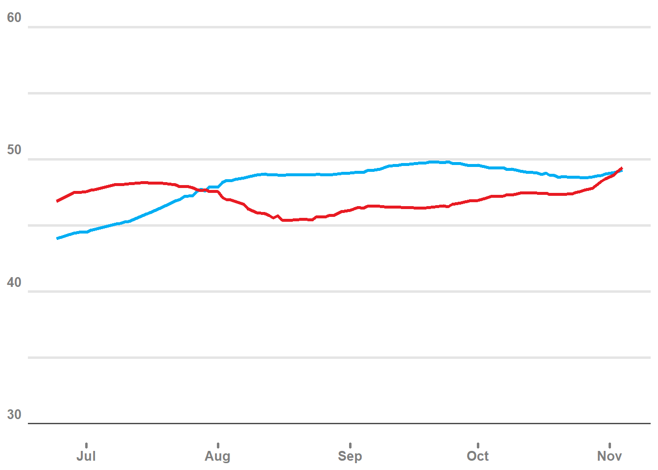
plot1<-
test %>%
  group_by(party, end) %>%
  summarise(across(ymin:ymax, mean)) %>%
  ggplot(aes(x = end)) +
  geom_line(aes(y = median, group = party, color = party), linewidth = 1.2) +
  scale_color_manual(values = c("#00AEF3","#E81B23")) +
  scale_fill_manual(values = c("#00AEF3","#E81B23")) +
  scale_y_continuous(limits = c(30, 60)) +
  geom_hline(yintercept = 30, color = 'grey20') +
  theme_minimal() +
  theme(legend.position = "none",
        panel.grid.major.x = element_blank(),
        panel.grid.minor.x = element_blank(),
        panel.grid.major.y = element_line(color = "grey90", linewidth = 1 ),
        panel.grid.minor.y = element_line(color = "grey90", linewidth = 1),
        axis.ticks.x = element_line(lineend = "round", linewidth = 1, color = 'grey50'),
        axis.title = element_blank(),
        axis.text = element_text(size = 10, color = 'grey50', face = 'bold'),
        axis.text.y = element_text(vjust = -0.5))
plot1

# labels for end points
end_labels <- test %>%
  filter(end == max(end)) %>%
  group_by(party) %>%
  slice(1)


# w/o error bars
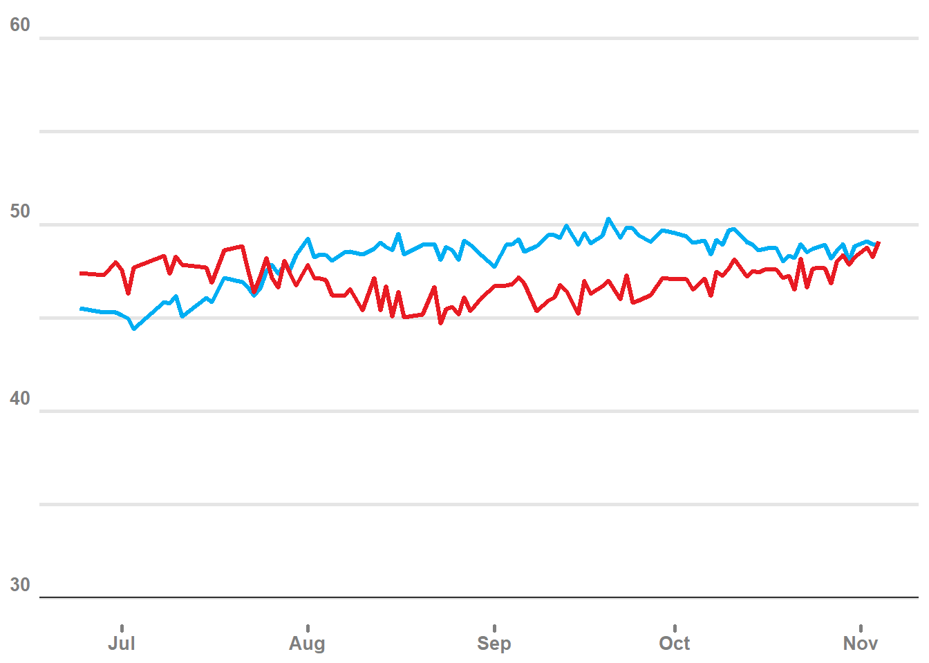
plot1 +
  geom_point(data = all_polls_df, aes(x = end, y = pct, color = party, fill = party), shape = 21, size = 2, alpha = .2)

# add point sizes and label
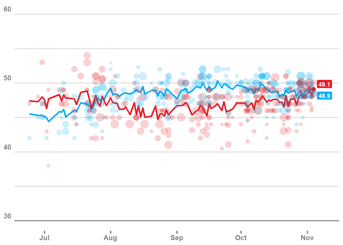
plot1 +
  geom_point(data = all_polls_df, aes(x = end, y = pct, color = party, fill = party, size = pop), alpha = .2) +
  geom_point(data = end_labels, aes(x = end, y = median, color = party), size = 2.5) +
  geom_label(data = end_labels, aes(x = end, y = median, label = round(median,1), fill = party), color = 'white', fontface = 'bold', nudge_x = 5, nudge_y = c(-.75,.75), size = 3.2)

 # facet plots
plot1 +
  geom_point(data = all_polls_df, aes(x = end, y = pct, color = party, fill = party, size = pop), alpha = .2) +
  geom_ribbon(aes(ymin = ymin, ymax = ymax, group = party, fill = party), color = 'white', alpha = .2)


# difference on max data
raw_dem <- stack_extract_posterior_predictions_naive(fit2.1, fit2.1s, weights = weights, return = "raw")
raw_gop <- stack_extract_posterior_predictions_naive(fit2.2, fit2.2s, weights = weights, return = "raw")


# compute dem margin based on most recent 10 days worth of polls
dem_margin <- raw_dem / (raw_dem + raw_gop)

max_date <- max(pred_dem$end)
date_idx <- seq.Date(from = max_date,by = "-1 day",length.out = 10)
T <- as.numeric(rownames(pred_dem[pred_dem$end %in% date_idx, ]))

mean(apply(dem_margin[,T], 1, function(x) mean(x > .5)))

# 95% CI and mean
# predicted share of 2-party vote
mean(apply(dem_margin[,T], 1, quantile, probs = c(0.025)))
mean(apply(dem_margin[,T], 1, mean))
mean(apply(dem_margin[,T], 1, quantile, probs = c(0.975)))

# predicted % times that dem candidate wins popular vote
# NOT the same as winning the election !!!
mean(dem_margin[,T] > .5)

hist(dem_margin)


Comments